Computational Optics
Characterizing Sensors
How we measure what a phone camera's sensor actually responds to, one narrow band of light at a time, and what the measurements show.

Everything else in this work rests on knowing how a particular sensor turns light into numbers. Datasheets don't tell you that for a phone camera, and the processed images a phone hands to apps hide it. So we measure it.
The rig
The characterization rig is a chain of standard spectroscopy instruments:
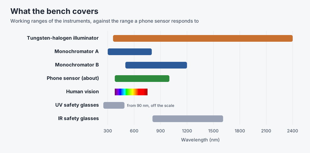
- A tungsten-halogen illuminator. A stable, broadband source with a smooth, continuous spectrum from the ultraviolet into the infrared. It's switched on 10 to 15 minutes before a session so its output settles.
- Monochromators. A monochromator spreads the lamp's light with a diffraction grating and lets a slit pass only a narrow band. We use two manual units, one covering 300 to 800 nm and one covering 500 to 1200 nm, so a sweep can run from near-ultraviolet to near-infrared.
- Slit sets. Interchangeable 100-micron slits set the bandwidth and throughput, and SMA adapters match them to the monochromators. Slit width stays fixed and logged for a whole sweep.
- Fiber-optic patch cords. Fibers are optimized for a range of light, so we keep separate UV/visible and visible/near-infrared cords.
- Long-pass filters. A set of OD 2 filters with cutoffs between 400 and 850 nm block everything shorter than their edge. They suppress stray light, sort out higher diffraction orders from the grating, and give us known edges to sanity-check the sweep.
- A diffuse reflectance standard. A white Spectralon target reflects about 99 percent of the light that hits it, almost perfectly evenly in every direction and almost equally at every wavelength. The camera looks at the target, not the beam, so every pixel sees the same light.
The procedure
- Lock the camera. RAW capture (DNG or ProRAW on iPhone), manual focus, fixed ISO and exposure, white balance locked, noise reduction off. Exposure is set so the brightest wavelength doesn't clip, then left alone.
- Shoot dark frames. With the lens capped, ten frames whose median becomes the per-channel dark level.
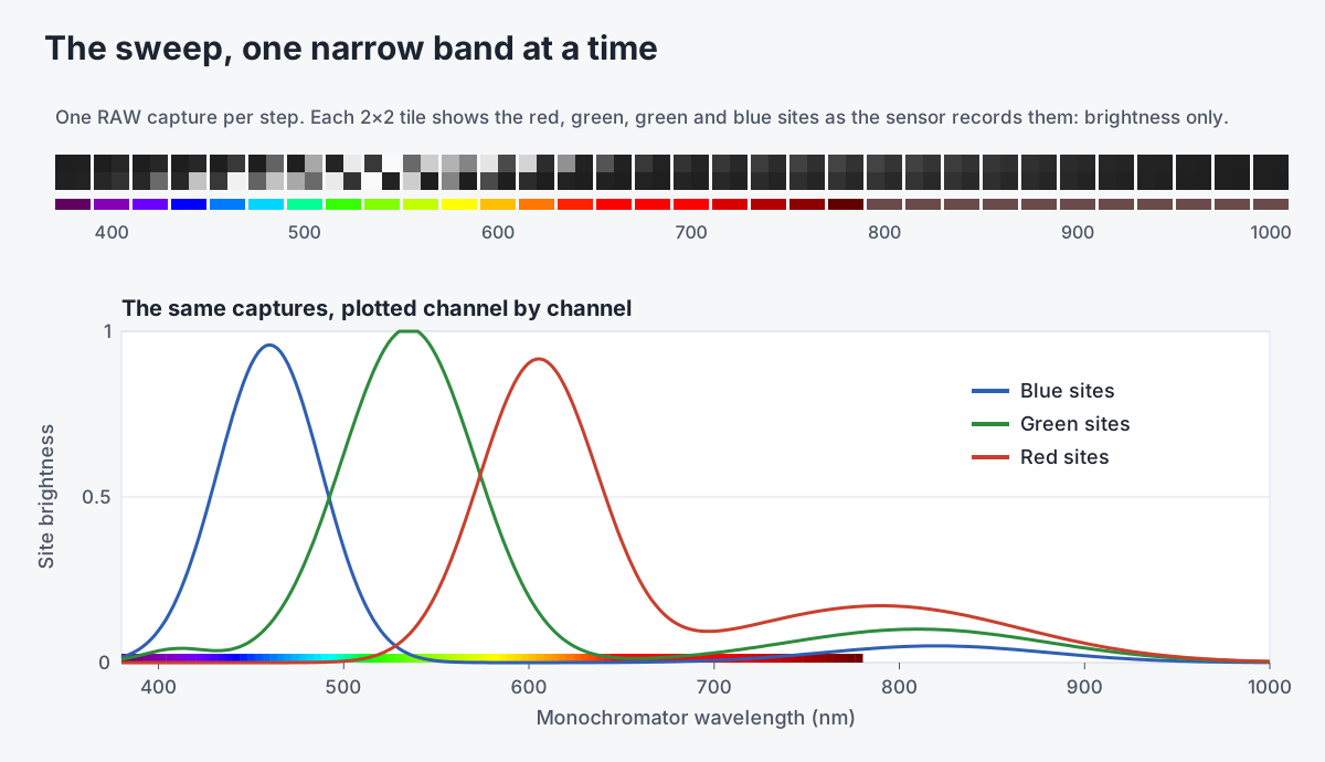
- Sweep. Step the monochromator in 5 to 10 nm increments across the range the source and grating support, roughly 380 to 1000 nm. At each step, record the wavelength, slit width, exposure, ISO and temperature, and capture three RAW frames.
- Check the edges. Shoot through the long-pass filters to confirm the tails behave as the sweep says they should.
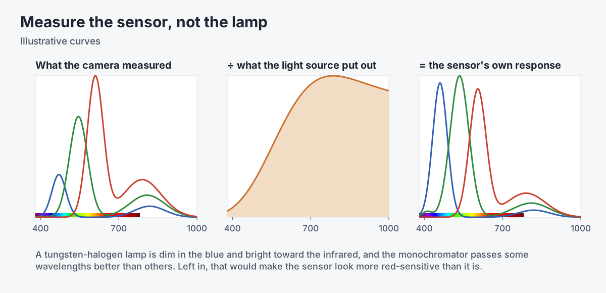
- Remove the source. Divide out the lamp and monochromator throughput, measured with a spectrometer or taken from the vendor curve, so the result describes the sensor rather than the light.

Staying in RAW
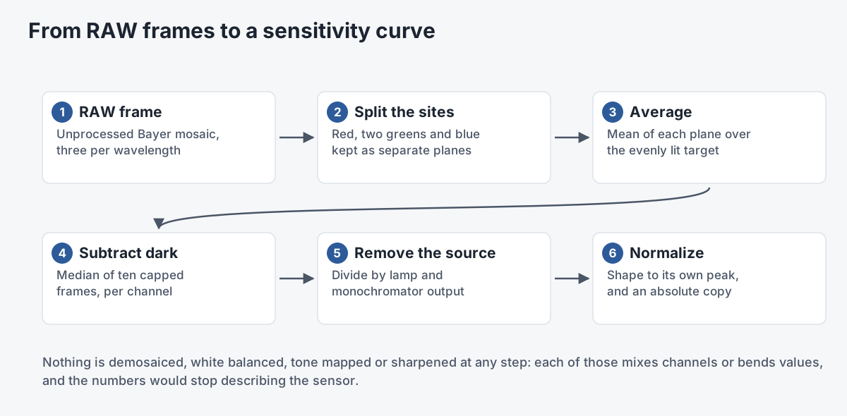
All of this happens on the raw Bayer mosaic. Demosaicing, white balance, color matrices, tone curves, noise reduction and sharpening each mix channels or bend values in ways that destroy the physical meaning of the numbers.

We split the mosaic into its red, two green and blue sites, take the mean of each, and subtract the dark level. Each channel's curve is kept both in absolute terms and normalized to its own peak, so we can compare shapes across devices and keep real sensitivities for modeling.
What the curves show

We look for three things:
- Where the peaks sit. Typically blue around 450 to 470 nm, green around 540 to 560 nm and red around 600 to 620 nm, varying with the sensor and its filters.
- How much the channels overlap. Overlap is what lets three channels encode more than three independent numbers' worth of spectral shape.
- What leaks. A rising red tail, and often a green one, past about 650 nm into the 800 to 900 nm range, and a small but non-zero response below 400 nm where the lens glass allows it. This out-of-band response is the extra signal the method exploits.
The fitted curves, smoothed with a basis such as B-splines for each channel, become the sensor's spectral sensitivity function. That function is used twice later: to choose the right model for a device, and inside training, where predicted spectra are pushed back through it to check they would have produced the RAW values the phone recorded.
A finding about phones
Getting RAW data out of phones turned out to be uneven. Native sensor data from the rear cameras is broadly available on both iOS and Android, with varying quality but usually good enough. Front cameras are a different story: many devices won't deliver raw Bayer data from them at all, a restriction that appears to be built into the hardware or firmware. Since that changes what each camera can contribute, we characterize front and rear cameras separately on every device.
Profiles, not one-offs
A characterization can belong to a single unit, keyed to its device identifier, or to a model, averaged over several units with the spread between units recorded. Profiles carry metadata about the lens, the infrared-cut filter and firmware, so a new capture can pick the closest profile or interpolate between profiles. The provisional also covers lighter-weight paths: calibrating with only broadband light and a set of targets of known reflectance, starting from simulated responses computed from filter and silicon properties, and refining a profile in the field from a quick capture of a gray card and one narrowband LED.
Related work
-

ISO-5 Optical Cleanroom
A cleanroom lab built to turn phone cameras into spectral instruments.
-
CameraSmartPlate
A camera plate that knows where it is, for tracking, virtual production and NeRF capture.
-
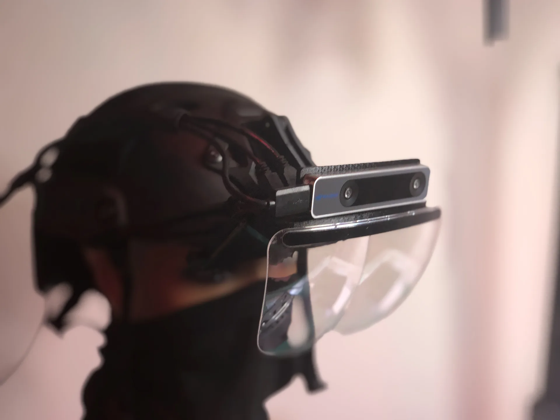
HoloFlect
A modular, upgradeable AR headset platform built for enterprise.
-
xR Ecosystem
A modular, device-agnostic programming interface for mixed reality.