Computational Optics
How It Works
The invention in plain language, from what a phone sensor actually measures to how a learned mapping turns RAW pixels into spectra.
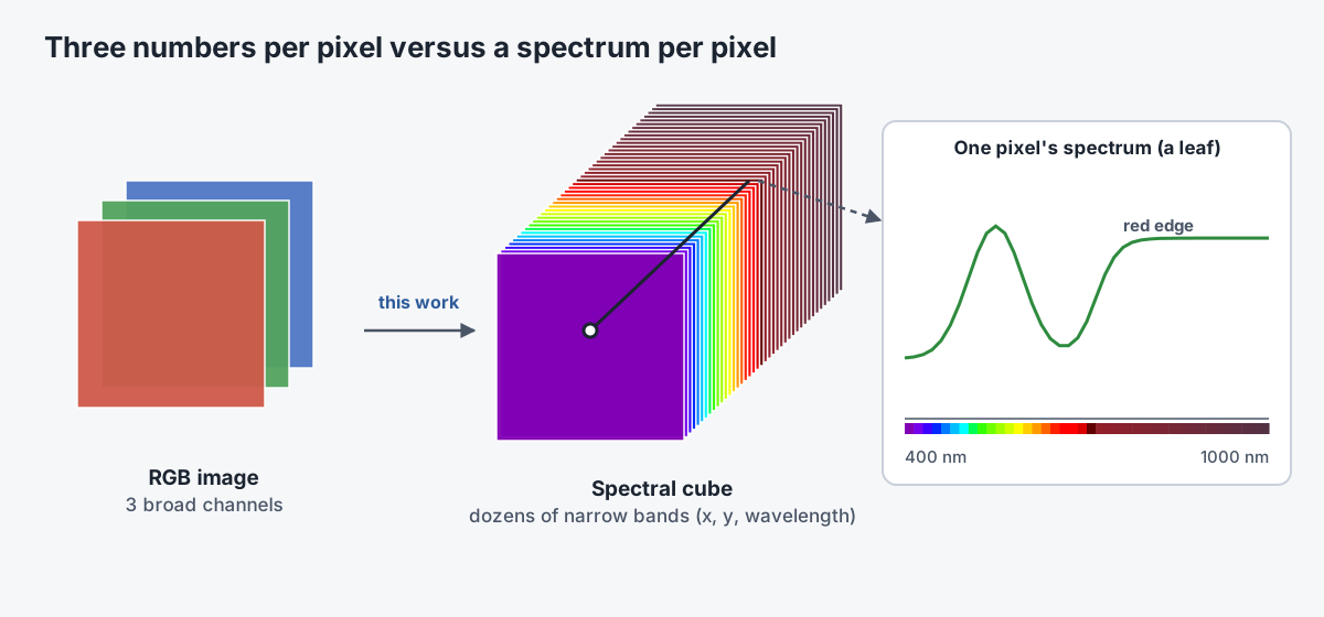
This page explains the method described in our provisional patent application, "Systems and Methods for Generating Hyperspectral Image Data From Commodity Imaging Sensors", for a reader who knows cameras but isn't an optics specialist.
Three numbers versus a spectrum
Light reflected from an object is a mixture of wavelengths, and the mixture is a fingerprint of the material. A spectrum records how much light there is at each wavelength.
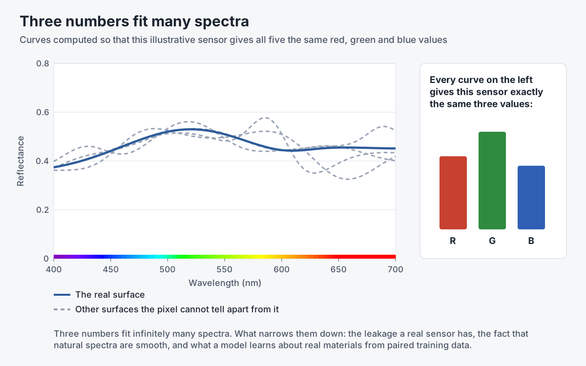
A color camera doesn't record that. Each photosite sits under a red, green or blue filter, and reports one number: the total light that got through its filter. Three numbers per pixel, after demosaicing, is enough to reproduce color for human eyes, because human eyes also only have three kinds of color receptor. It isn't enough to tell two materials apart when they happen to produce the same three numbers.
A hyperspectral image keeps the fingerprint. The patent application defines it simply: image data sampled at more than three spectral bands, typically narrow and evenly spaced over a continuous range. Stack those bands and you get a spectral cube, with two dimensions for the image and one for wavelength. Every pixel in the cube is a full spectrum.
What the phone already knows
The red, green and blue filters on a phone sensor aren't clean, separate windows. Their passbands overlap, each lets through some light far from its nominal color, and the silicon underneath stays sensitive well into the near-infrared. Phones add an infrared-cut filter, but it attenuates rather than erases. The patent's starting observation is that "the actual spectral sensitivity of these sensors and their color filters is often broader and more complex than the nominal red, green, and blue passbands."
That complexity is a nuisance for photography. For us it's information. If you know exactly how each channel of a particular sensor responds to each wavelength, the three channel values carry more about the incoming spectrum than three ideal filters would, and a model can use spatial context, priors about real-world materials and the sensor's physics to estimate the rest.
Stage one: characterize the sensor
We first measure the sensor's spectral response. A broadband lamp feeds a monochromator, which passes one narrow band of wavelengths at a time onto a calibrated white target. The phone photographs the target in RAW at each band, with every automatic feature off. Plotting each channel's response against wavelength gives its spectral sensitivity function, leakage and all.
The result is a characterization profile, stored for a specific device or, by measuring several units of a model, for the model as a whole. Metadata such as lens, infrared-cut filter and firmware version travels with it, so the right profile can be chosen or interpolated later. Characterizing Sensors covers the procedure step by step.
Stage two: capture paired data
Next we build the training set. The phone captures RAW images of scenes while a reference system, a hyperspectral camera, an imaging spectrometer or a point spectrometer, measures the same scene regions at the same time or close to it. Checkerboards, fiducial markers, fixtures and software registration line up each phone pixel with its reference spectrum.
Scenes range from calibration targets to natural scenes to application-specific material sets: foliage, skin, textiles, paints, food. Lighting and environment vary on purpose, so the model learns the material, not the lamp.
Stage three: learn the mapping
With pairs of RAW values and true spectra, we derive an inverse mapping from sensor space to spectral space. The patent covers the whole range of ways to do this: linear and non-linear regression, neural networks (multilayer perceptrons, convolutional networks, transformers), kernel methods such as Gaussian processes, and hybrid models that build in the known sensor physics.
The model's inputs can include each pixel's raw values, its spatial neighborhood, and capture metadata such as device model, exposure and estimated illuminant. Its output can be a continuous spectrum per pixel, a fixed set of bands, or a measurement derived from the spectrum, such as a vegetation index or a material score. Training compares predicted spectra to reference spectra with spectral distance measures, optionally weighting some wavelengths more than others or adding a task-specific loss. Learning the Spectrum goes deeper.

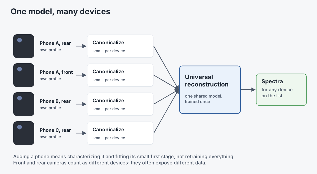
One arrangement in the application is worth singling out. The mapping can be split into two stages: a device-specific "canonicalization" step that converts one phone's raw responses into a device-invariant intermediate signal, and a universal reconstruction step that turns that signal into spectra. Adding a new phone then means characterizing it and fitting the first stage, not retraining everything.
Stage four: deploy
In use, the device captures RAW or minimally processed data, picks the right profile and model variant from its metadata, optionally estimates the lighting, and applies the mapping to every pixel. The computation can run entirely on the device, entirely on a server, or split, with preprocessing on the phone and reconstruction in the cloud.

When latency or power matters, the system can predict fewer bands, predict a coarser cube and sharpen it with super-resolution, or skip full spectra and compute only the index an application needs. The mapping can also keep improving: as new paired data or in-field calibration captures arrive, it can be refined and re-calibrated, for example to follow a sensor as it ages.
What the application covers
Beyond the core method, the provisional describes a wide set of variations: monochrome sensors with switched filters or illumination, sensors with non-Bayer filter arrays such as RGBW, calibration from natural light or from simulated sensor responses, models that estimate the illuminant and the surface reflectance together, models that report their own uncertainty, compact spectral bases instead of full curves, federated training that never moves raw images off devices, synthetic training data from rendering engines, and multi-frame or depth-assisted capture for 3D spectral reconstruction. Several of these are the subject of Research Directions.
Related work
-

ISO-5 Optical Cleanroom
A cleanroom lab built to turn phone cameras into spectral instruments.
-
CameraSmartPlate
A camera plate that knows where it is, for tracking, virtual production and NeRF capture.
-
HoloFlect
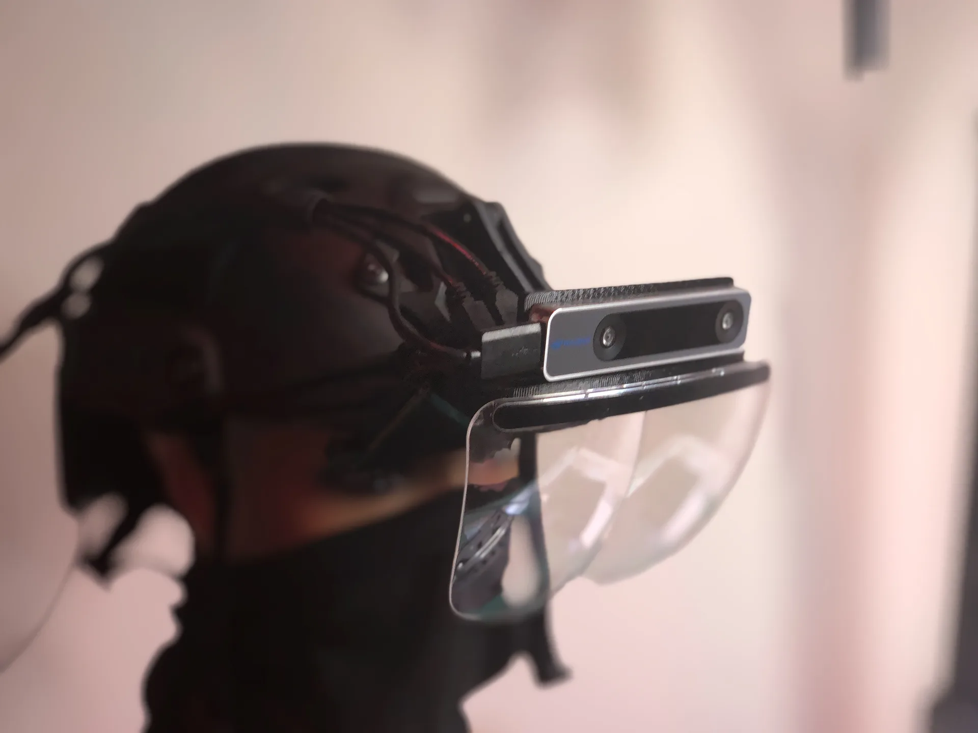
A modular, upgradeable AR headset platform built for enterprise.
-
xR Ecosystem
A modular, device-agnostic programming interface for mixed reality.