Computational Optics
Learning the Spectrum
How we build paired training data, calibrate two very different cameras against each other, and train a model that turns RAW pixels into physically plausible spectra.
A characterized sensor tells us what the phone can see. To turn that into spectra, the model needs examples: many scenes where we know both what the phone recorded and what the true spectrum was. This page covers how we collect those examples and what the model does with them.
Two cameras, one view
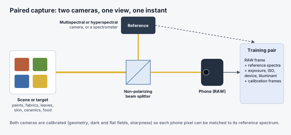
The reference is a camera that measures spectra directly. The rig is designed to pair a phone with a multispectral reference camera, such as a JAI Fusion prism camera, behind a non-polarizing cube beam splitter. The splitter sends half the light from the scene to each camera, so both see the same view at the same instant, with no parallax and no chance for the light to change between shots.
Both cameras ride on a rigid mount. We specified a custom six-degree-of-freedom fixture, printed in engineering resin over several design iterations, that holds two cameras on a robot arm and lets each be adjusted independently, so the pair can be aligned once and then moved around a scene as a unit. We wrote our own control software for the arm.
Calibrating the pair
Two very different cameras have to agree on where things are, how bright they are and how sharp they are before their pixels can be paired:
- Geometric. Each camera's lens is calibrated with a checkerboard, and the transform between the two is solved, so reference spectra can be warped onto the phone's frame. Dense optical flow refines the match.
- Radiometric. Dark frames at each exposure and gain, and flat fields from an integrating sphere or uniform panel, for both sensors.
- Spectral. The reference camera's band centers and widths are verified, and the phone's channel sensitivities come from sensor characterization.
- Sharpness. A slanted-edge chart gives each camera's point spread function, and the sharper image is blurred to match the softer one so the model isn't asked to invent detail.
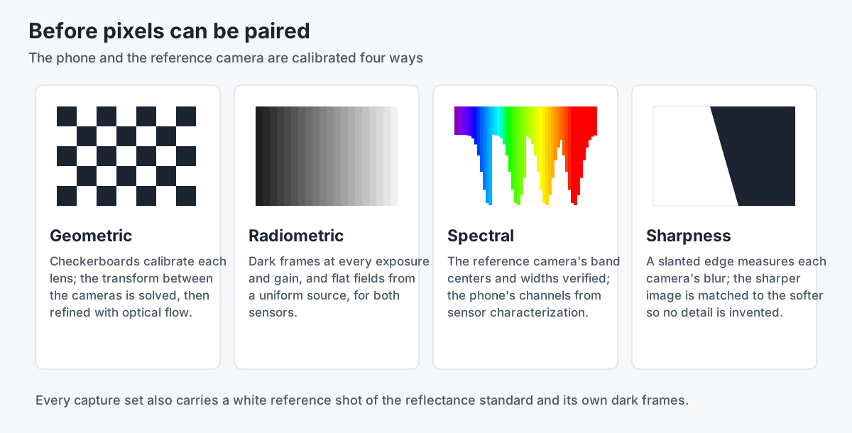
Every set also includes a white reference shot of the reflectance standard and dark frames. Reference data is converted to reflectance and resampled onto a uniform 5 to 10 nm grid.
What we photograph
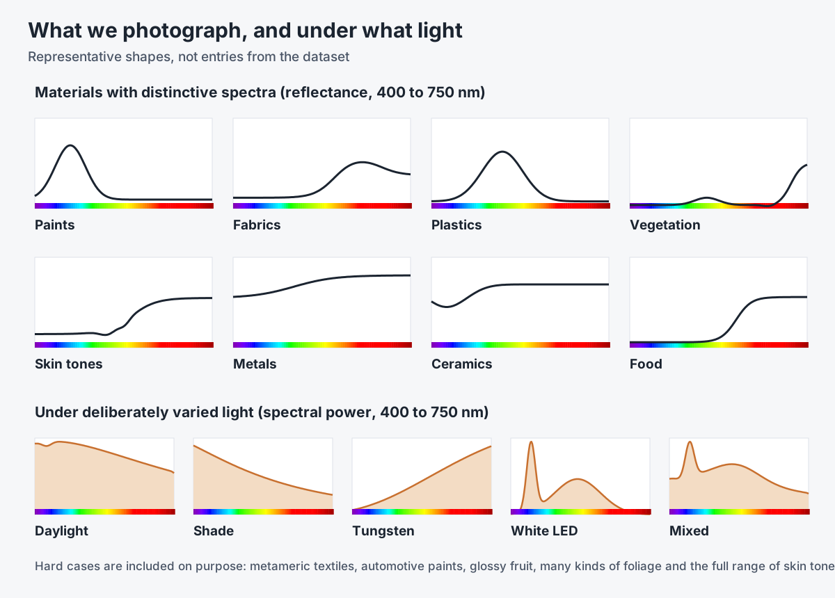
The dataset design calls for hundreds to a few thousand unique scenes, indoors and out, chosen for materials with distinctive spectra: paints, fabrics, plastics, vegetation, skin tones, metals, ceramics and food. The hard cases are included on purpose: metameric textiles that match in color but not in spectrum, automotive paints, glossy fruit, many kinds of foliage, and the full range of skin tones.
Lighting varies as deliberately: daylight across a range of color temperatures, tungsten, LEDs with different spectra, shade and mixed light, logged with a small spectrometer when possible. Exposures are bracketed to avoid clipping, and glossy subjects are shot with and without crossed polarizers so reflections can be separated from the material underneath.
Each capture is stored as a DNG with full metadata and a JSON sidecar, the reference data in a standard hyperspectral format with band centers and units, and a per-scene manifest that ties both captures to their calibration frames and lighting log.
The model
The model reads the phone's RAW mosaic directly, either as a single plane with a channel mask or packed into four quarter-resolution planes, along with exposure, ISO and an estimate of the illuminant. A U-Net or HRNet backbone extracts spatial features, and a per-pixel spectral decoder produces 31 to 61 bands.
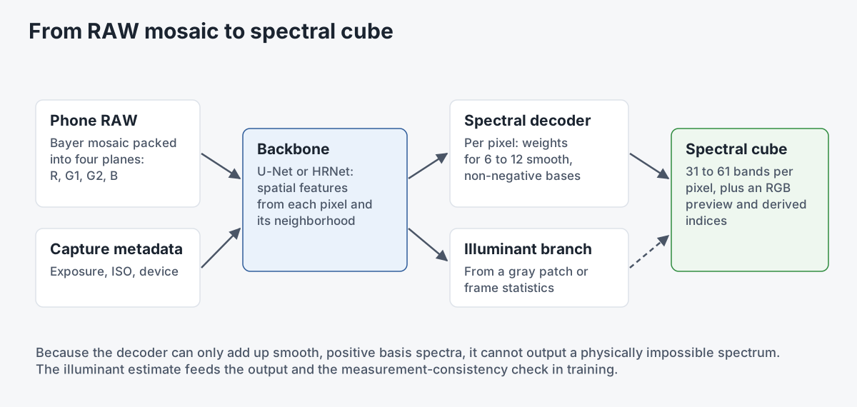
Two decoder designs are in play. One predicts coefficients for a small set of smooth, non-negative basis spectra, typically 6 to 12, and sums them. The other is a small per-pixel network with a non-negativity constraint. The basis approach builds in a useful prior: real reflectance spectra are smooth and low-dimensional, so a model that can only produce smooth, positive spectra can't produce physically impossible ones.
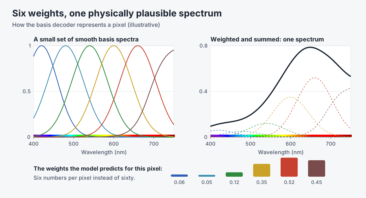
A separate small branch estimates the illuminant's spectrum from a gray patch or the frame's overall statistics.
Checking the answer twice

Training compares the predicted spectrum with the reference in two ways, an error per band and the spectral angle, which measures whether the shape is right regardless of brightness. A smoothness term along wavelength and a non-negativity constraint keep the output physical.
The more distinctive check is measurement consistency. Because we know the phone's channel sensitivities and the illuminant, we can push the predicted reflectance back through the camera, multiplying by the light and by each channel's sensitivity and integrating, and ask whether it reproduces the RAW values the phone actually recorded. A spectrum that matches the reference but couldn't have produced the observed pixels is wrong somewhere, and this loss catches it.
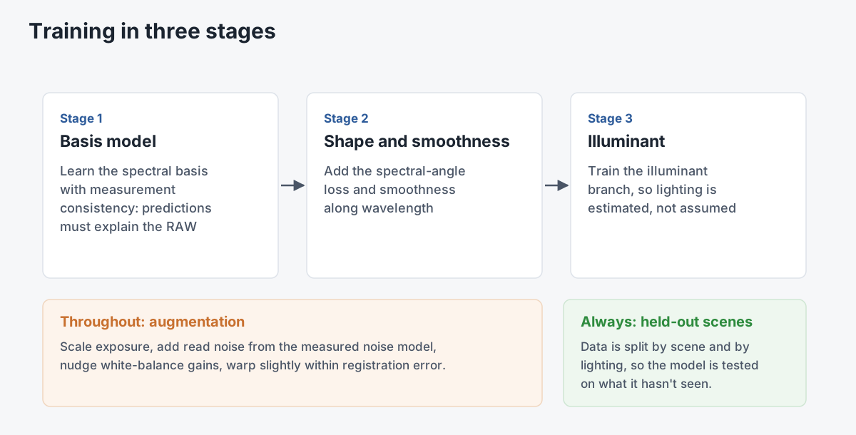
Training follows a curriculum: first the basis model with measurement consistency, then the spectral angle and smoothness terms, then the illuminant branch. Augmentations scale exposure, inject read noise from the calibrated noise model, nudge white-balance gains and add small warps within registration tolerance. Data is split by scene and lighting, so the model is always tested on scenes it hasn't seen.
How we judge it
- Per-band error and spectral angle on held-out scenes.
- Material classification accuracy using predicted spectra against a reference library.
- Re-rendered RAW compared with measured RAW.
- Field tests: vegetation and photochemical indices computed from predicted bands against the same indices from the reference camera.
Honest limits
Phone sensors are weak below 400 nm and above about 700 nm, because of the infrared-cut filter and the microlenses. Gains are largest between roughly 420 and 750 nm; beyond that, much of what the model predicts comes from priors, and we report confidence per band rather than pretending otherwise.

Mixed lighting and strong specular highlights break the simple reflectance model, which is why polarized captures and illuminant estimation are built into the capture design. And registration with scanning reference cameras is fragile on moving scenes, which is why we prefer a snapshot reference camera behind a beam splitter.
The deliverable at the end of this pipeline is an inference package: RAW in, spectral cube out, with a fast RGB preview and derived indices, exportable to Core ML or TensorRT for on-device use.
Related work
-

ISO-5 Optical Cleanroom
A cleanroom lab built to turn phone cameras into spectral instruments.
-
CameraSmartPlate
A camera plate that knows where it is, for tracking, virtual production and NeRF capture.
-
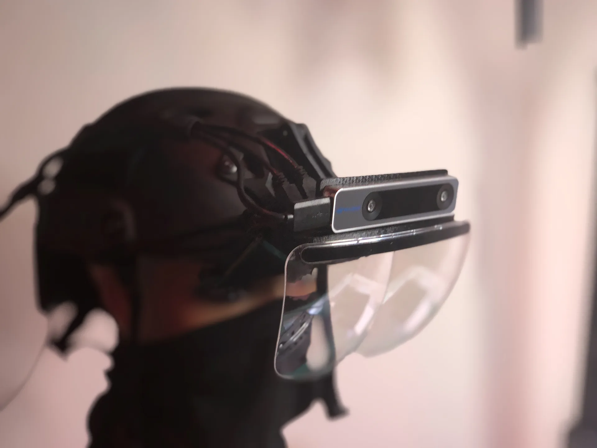
HoloFlect
A modular, upgradeable AR headset platform built for enterprise.
-
xR Ecosystem
A modular, device-agnostic programming interface for mixed reality.